Achieving spatial representation for arbitrary shapes efficiently using a computer is non-trivial. This is especially true if you want minimal memory usage and fast operations (e.g. testing whether a point is inside or outside a shape, union/intersection/difference of pairs of shapes) on them – especially important in large-scale MMO game design. This gets even harder in more than two dimensions. In this post we discuss the research we’ve been doing at Hadean and invite you to try our C++ open source library.
Approaches
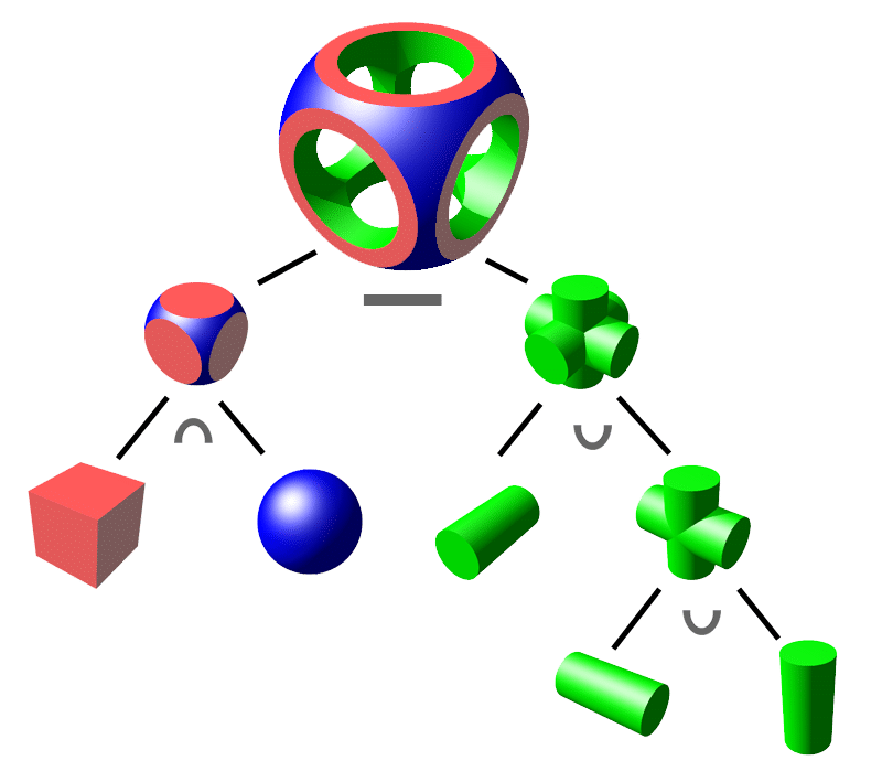
One approach for spatial representation of complex shapes is from simple primitives, such as spheres and boxes. The primitives are combined using an operation between each pair, forming a tree with the leaves being simple shapes and the internal nodes being operations to combine them. The root of the tree is the final shape. To implement operations on the total shape, you would recursively apply them through the tree. This is known as Constructive Solid Geometry (CSG).
Another approach for spatial representation is to break up your ‘world’ into a bitmap, with each bit saying whether or not the shape exists in that position. Although operations on this representation can be fast and use little memory for small or shapes with little detail, it scales very poorly with large or more detailed shapes, and scales extremely poorly in more than two dimensions. If you know Minecraft, then you know this approach. Minecraft uses a 3D “bitmap” of voxels to store the world data. The only difference is that Minecraft has a huge variety of voxel values (dirt, stone, etc), where a shape bitmap would only have inside/outside values.
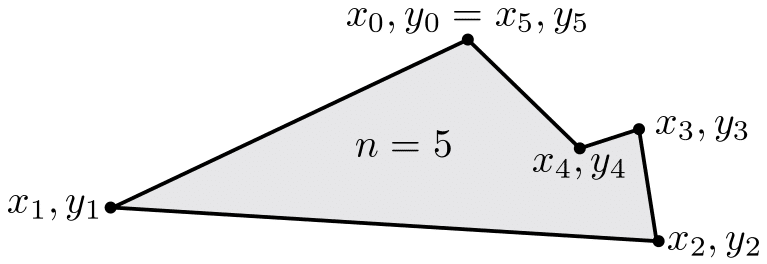
A third approach is a boundary spatial representation, which stores vectors or planes (or hyperplanes) that are the boundary between the inside and outside of the shape. This is very commonly used for rendering meshes. Memory usage is proportional to the complexity of the shape, but the operations on the shape (apart from for rendering it to a screen) are not very fast. To implement the operations is also a non-trivial task, libraries for this do exist, but, again, extending this to higher than two dimensions is a hairy task.
Taking some inspiration from all three of these approaches, we might say we’d like an interior (or volume) representation (as opposed to a boundary or surface representation) for fast and simple operations. And we’d like a representation that scales well in memory usage and operation speed given the complexity of the input shapes.
A sparse hierarchical grid fulfills both of these nicely. As in the bitmap representation, membership of the shape is defined on a grid. But unlike the flat bitmap, we do not store the same level of detail over the whole shape or world.
Octrees and Quadtrees are the main example of sparse hierarchical grids. They take a 2D (or 3D for an Octree) space, and divide it into four (or eight) child squares (cubes) that perfectly cover the parent without overlapping with each other. The child squares are half the length of one of the sides of the parent, dividing the space exponentially – in 2D one becomes four becomes 16 becomes 64 etc.
However, for many use cases, octrees and quadtrees are too heavyweight, both in storage space and operation speed. They both scale well, ideally, providing O(log(N)) accesses, and O(log(N)) operations. But for small N (~200), the storage of pointers, nodes, leaves in the tree is far too much overhead.
An alternative way to define an octree is by just storing the leaf nodes as their position along a space filling curve, along with either a size/length (often stored in log2 form) or an end position along the same space filling curve.
Space Filling Curves
An elegant way to implement sparse hierarchical grids is using a space filling curve. Space Filling Curves are lines that curve their way through the space in a certain pattern that fills up the space when taken to enough detail.
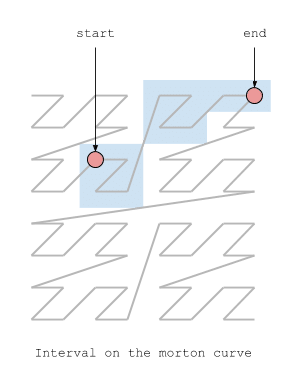
The link between space filling curves and sparse hierarchical grids is that if you number every point in space along a single number line you can define regions of space using only a start and end point on that number line.
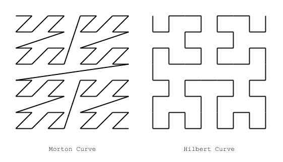
There are many space filling curves, but the two most well known and widely used are the Hilbert curve, and the Morton curve (also known as the Z-Order curve). The Hilbert curve has good locality properties, meaning it tends to put nearby points in N dimensional space close to each other in 1D curve space. Morton curves have good-ish locality properties, but where they really shine is their simple and fast encoding and decoding ability: to produce a morton encoded position, you just interleave the bits of the coordinates of the position.
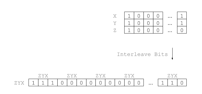
The problem with representing regions of space as a start and end point on a space filling curve, is that you can’t represent all possible shapes. In order to do that, you’d need an infinite list of regions (for approximation, a finite list will do) that together make up the shape. This is what we refer to as a Morton region. So, the morton interval is just a start and end point on the 1 dimensional morton curve, the morton region is a sorted, non-overlapping list of these intervals. Morton regions are also known as a Linear Octree. See also the section “Linear (hashed) Octrees”).
Morton Regions in Spatial Representation
The conversion from an input shape to a morton region is generally done recursively, by doing an intersection test of the input shape against the largest square of the octree, and then repeating for the child squares that are overlapping. This can be limited by a certain accuracy you want to achieve in the representation. There are also specific input shapes which are easier (and faster) to convert.
A good example of this is an AABB (axis-aligned bounding-box). It is only possible on the morton curve (so far no other fractal curves have this property for AABBs) to calculate exactly where the curve intersects with the AABB edges. The terminology around these functions is confusing and overlapping because they aren’t widely talked about, although they are commercially used in some databases and geospatial information systems. Some names of these functions are BigMin/LitMax, NextJumpIn, GetNextZ-Address.
This list of morton intervals representation is very simple to perform operations on, because it is a one-dimensional line. If you can do a union of two intervals on a 1D line, the space filling curve means you can do them in N dimensions with the same code!
Morton regions require much less space than an equivalent bitmap, are faster for querying and processing than boundary representations like edge lists, and are faster than hierarchical representations like CSG or Octrees/Quadtrees because they don’t require traversing a tree, usually following pointers or indices and give much easier cache locality by keeping the list of intervals sorted.
To keep things fast, you would maintain that the list is always sorted by the start position of each interval along the space filling curve. This means you can iterate sequentially through the two lists in order. So, combining two or more shapes using boolean set operations can be implemented very simply in O(M+N) time, where M and N are the length of the two input lists.
In order to make this implementation more useful, you may want a map type, which associates one arbitrary domain to another. This spatial map can efficiently index from N dimensional space to another arbitrary domain (even process identifiers!). This is done by templating the morton region with a type T that is attached to each morton interval and carried with it through the set operations.
At Hadean, we use this Morton region set/map type as the core of Hadean Simulate. It powers the complex games and scientific simulations that we perform at incredible scale and resolution.
Finally, we are pleased to make our research available in an open source N dimensional spatial processing C++ library libzinc. You can find the library on GitHub and we welcome your involvement.